Edit a Physical View
|
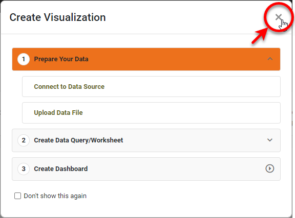
If you see the ‘Create Visualization’ dialog box, press the ‘Close’ button
|

To modify an existing physical view, follow the steps below:
-
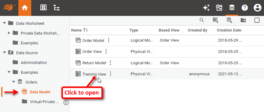
Press the top ‘Data’ button
 in the Portal.
 -
In the left panel, expand the ‘Data Sources’ folder.
-
Expand the data source for which the physical view is defined, select the ‘Data Model’ node, and click on the physical view to open it for editing.
-
To add tables and joins to the physical view, follow the appropriate steps in Create a Physical View.
-
To make other modifications, see the sections below and then press the ‘Save’ button
 to save the physical view.
Add Inline SQL
If you want to add custom business rules in your model without creating a new view in your database schema, you can create an inline embedded SQL view. This allows you to create a virtual “table” by embedding a SQL directly into the physical view.
| An embedded view may result in a different execution plan than a database view. You should test both options against your database. |
To create an inline view, follow the steps below.
-
Press the ‘Create Inline View’ button
 button.
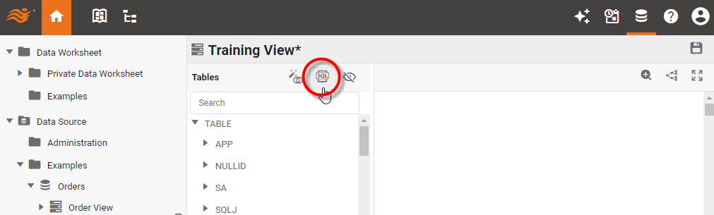
-
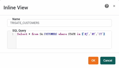
In the ‘Inline View’ dialog box, enter the view name in the ‘Name’ field, and type in the SQL query string into the ‘SQL Query’ field.
-
Press OK. This adds the inline view as a new table and places it into the physical view.
-
Join the inline view to other tables in the physical view as described in Create a Physical View.
-
Press the ‘Save’ button
in the top right to save the physical view.
Automatically Create Joins
When you are initially creating the physical view, it is often helpful to automatically create joins between many tables. To do this, follow the steps below:
-
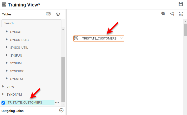
Select tables for the new physical view as described in Create a Physical View.
-
Press the ‘Auto Join Tables’ button
 at the top of the ‘Tables’ panel.
 -
Specify whether you want the joins to be constructed based on existing key relations or based on matching identical column names.
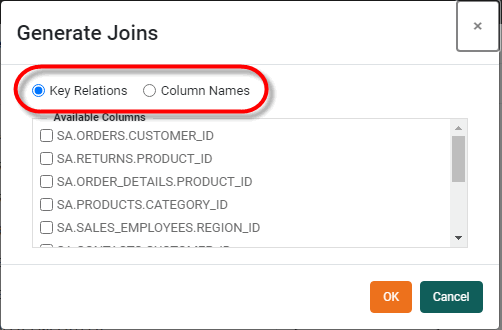
-
Select the key columns or column names for which you want to create joins, and press OK. This adds the specified joins into the physical view.
-
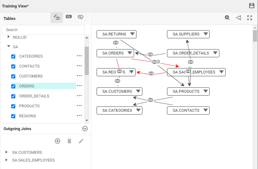
To simplify the appearance of the physical view and remove line crossings, press the ‘Auto Layout’ button
 in the toolbar.
Join paths that are displayed in red indicate the presence of a join cycle, which is an ambiguity in the join structure. See Resolve Loops for information on how to correct this problem. -
To modify the properties of a join, see Modify Join Properties.
-
Press the ‘Save’ button
in the top right to save the physical view.
Resolve Loops
| Identify Query Traps for physical view designs that can cause unexpected results. |
When a join path is displayed in red, this indicates that a join cycle (join ambiguity) exists.
+
There are several approaches to resolving join cycles:
-
Change one of the joins in the join cycle to a weak join. This specifies that this join relationship should be used only when it does not conflict with another join path, as for example when a query requests data only from the two tables joined by the weak join. To designate a join as a weak join, see Modify Join Properties. Weak joins appear as dotted lines.
-
Create an alias of a table in the join cycle. The alias table can be used in the physical view as a independent copy of the original table to break the join cycle while preserving the semantics of the join structure. See Alias Single Table for more information. An aliased table is indicated by a colored header. To display the name of the table that was originally aliased, hover the mouse over the alias table header.
-
Create an auto-alias of multiple tables in the join cycle. This is useful when the table that you want to alias has outgoing relationship links, and you therefore need to alias several “downstream” tables as well. See Alias Multiple Tables for more information.
Modify Join Properties
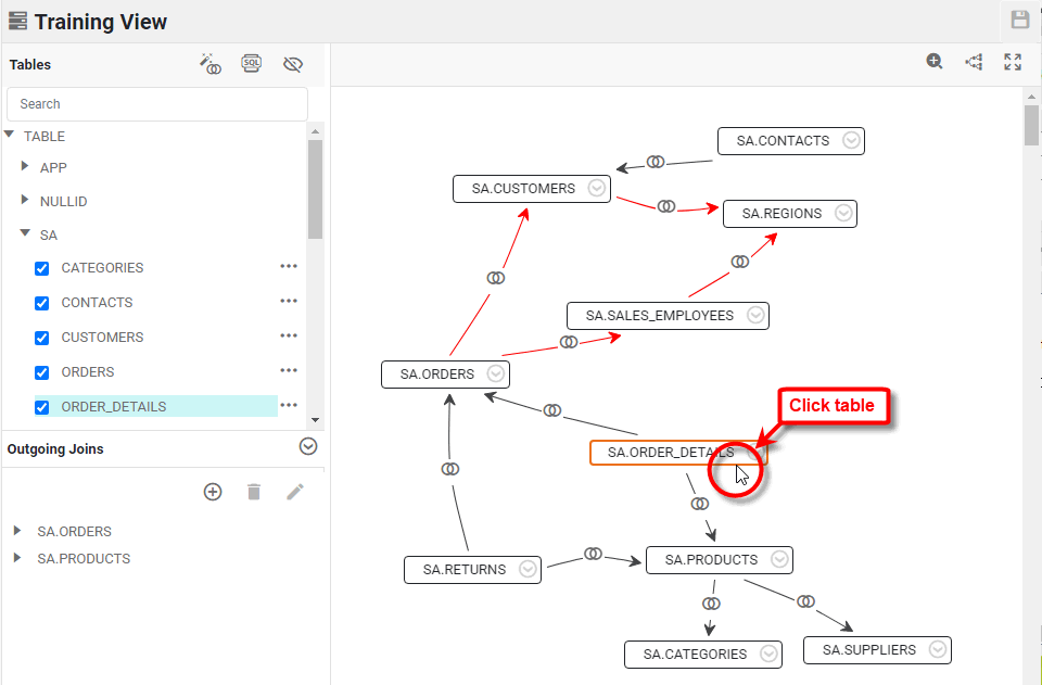
To modify properties of a join in the physical view , follow the steps below:
-
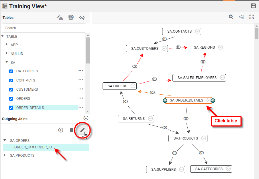
Click to select the table that has the outgoing join you want to modify.
-
In the Outgoing Joins panel, expand the selected table, click the join condition that you want to modify, and press the ‘Edit a join’ button
 .
.
-
Set the desired join characteristics in the ‘Edit Join’ panel.
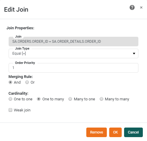
The following settings are available:
-
To delete the join, press the ‘Remove the selected join(s)’ button
 in the ‘Outgoing Joins’ panel.
 -
Press the ‘Save’ button
to save the physical view.
Alias Single Table
An alias table can be used in the physical view as a independent copy of the original table to break a join cycle while preserving the semantics of the model. (See Resolve Loops.) To create an alias for a single table, follow the steps below:
-
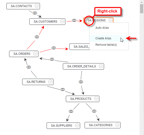
Right-click the table that you want to alias, and select ‘Create Alias’.
-
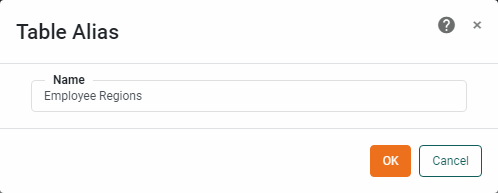
In the ‘Table Alias’ dialog box, provide a name for the alias table and press OK.
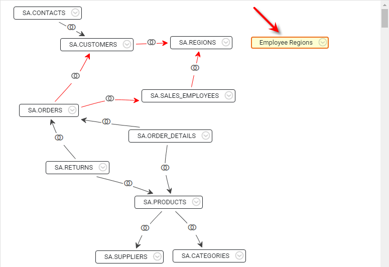
The new alias table is added into the physical view, highlighted in yellow. This table is identical to the original table, but can be used independently within the physical view.
-
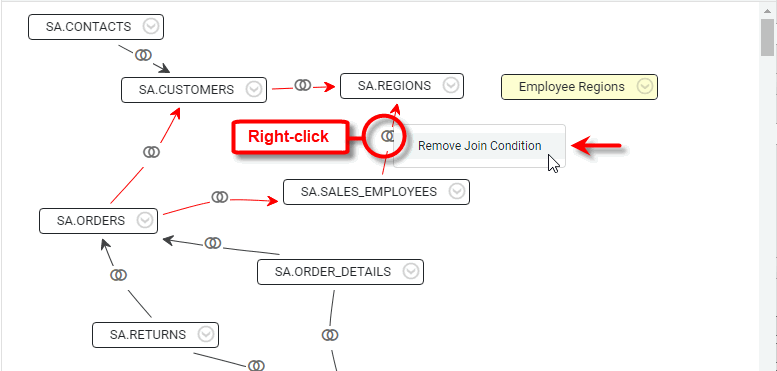
Click to select the original table (from which the alias was created), and delete the join that creates the cycle. See Modify Join Properties for information on how to delete a join.
-
Create a join to the new alias table. (See Create a Physical View for more information about how to add a join.)
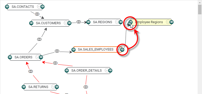
The alias table is now joined to the physical view as you specified, and the join cycle has been broken.
When you successfully break a join cycle, another join cycle might be highlighted. Only one join cycle is highlighted at a time. -
Repeat the above steps to address any additional highlighted join cycles.
-
Press the ‘Save’ button
to save the physical view.
Alias Multiple Tables
An alias table can be used in the physical view as a independent copy of the original table to break a join cycle while preserving the semantics of the view. (See Resolve Loops.) In some cases you may need to alias other “downstream” tables as well in order to break the cycle. The easiest way to do this is to use the auto-alias feature.
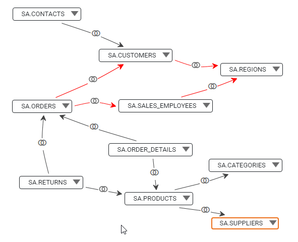
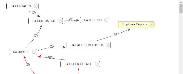
Consider a simple example in which you need to alias the table ‘PRODUCTS’ to resolve a join cycle.
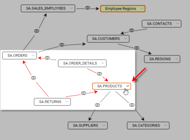
The joins highlighted in red indicate the presence of a cycle. Follow the steps below to break the cycle with an auto-alias:
-
Right-click the
PRODUCTStable in the diagram, and then select ‘Auto Alias’.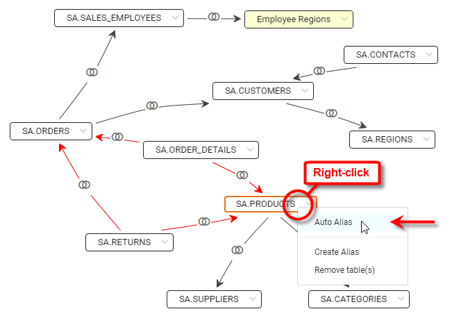
-
Check the ‘Enable auto aliasing’ box.
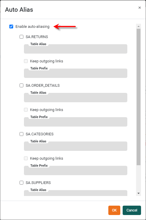
The dialog box lists all of the joins from the adjacent tables in the diagram.
-
Select the tables that provide the incoming joins to the
PRODUCTStable , in this case theORDER_DETAILSandRETURNStables.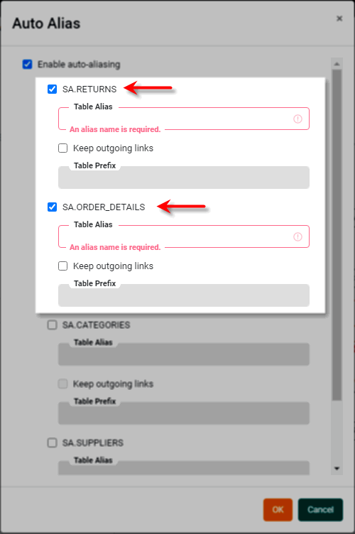
This designates the
ORDER_DETAILSandRETURNStables as providing the incoming joins to thePRODUCTStable. When thePRODUCTStable is auto-aliased, two copies of the table will be created. One copy corresponds to the incoming join from theORDER_DETAILStable, and the other copy corresponds to the incoming join from theRETURNStable. By splitting thePRODUCTStable into two aliases, the join cycle is eliminated. However, if only thePRODUCTStable is aliased, the cycle will simply reappear on theCATEGORIESandSUPPLIERStables. This is why in the next steps you will specify the ‘Keep Outgoing Links’ option. -
In the ‘Table Alias’ field for the
ORDER_DETAILStable, enter “Ordered Products”. -
Select ‘Keep Outgoing Links’ for the
ORDER_DETAILStable, and enter “Order” as the ‘Table Prefix’. This will cause the downstreamCATEGORIESandSUPPLIERStables to be aliased for theORDER_DETAILSjoin path as well. -
In the ‘Table Alias’ field for the
RETURNStable, enter “Returned Products”. -
Select ‘Keep Outgoing Links’ for the
RETURNStable, and enter “Return” as the ‘Table Prefix’. This will cause the downstreamCATEGORIESandSUPPLIERStables to be aliased for theRETURNSjoin path as well.
-
Press OK. Observe that the
PRODUCTS,CATEGORIES, andSUPPLIERStable have all been aliased, and this has successfully eliminated the join cycle.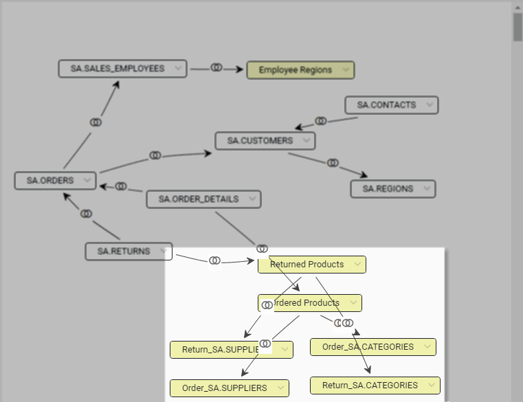
-
Press the ‘Save’ button
to save the physical view.
The new aliased tables in the physical view will appear among the tables available for constructing the logical model (see Logical Model). With the elimination of the cycle, there is no remaining ambiguity in the join structure.
When you design your logical model from a physical view with aliased tables, you must be careful when selecting fields as model attributes. For example, the Return_SA.SUPPLIERS table will in general return different data than the Order_SA.SUPPLIERS table when fields from these tables are used in a data model. Even though these two tables are identical aliases of the original SUPPLIERS table , they are joined to the other tables in different ways, which results in different data selections.
|
Identify Query Traps
A query trap is a construct in a physical view that can generate undesired query results which might confuse users or lead to inaccurate analyses. The sections below discuss query traps that you should avoid when you design a physical view.
| These traps usually do not occur in a star schema because this schema type has uniform 1-to-n relationships from dimension table to fact table, and all measures are located in the fact table. |
Loop Trap
Loops are multiple possible paths between tables in the physical view. Loops are always highlighted in red in the physical view. To resolve a loop trap, see Resolve Loops above.
Higher Level Aggregate Trap
It is always acceptable to aggregate measures at a lower level, but aggregating higher-level measures can cause erroneous results. This is the higher level aggregate trap.
What is a measure?A measure is generally used for aggregation, for example summation, averaging, correlation, etc., within a Crosstab, Chart, Text component, or Gauge. Adding a measure to the ‘Y’ region in a chart displays the computed aggregates by using locations on the Y-axis. Adding a measure to the ‘X’ region displays the computed aggregates by using locations on the X-axis. You can also display aggregates by using color, shape, size, or label. |
Consider the two tables below. The Order table contains an order ID field and the total amount of that order. The Item table contains an order ID field and item ID field. The Order table contains “higher-level” information than the Item table because it pertains to the entire order.
| Order |
|---|
Order_ID |
Order_Amount |
| Item |
|---|
Order_ID |
Item_ID |
The Order table has a one-to-many relationship with the Item table in this case, since there are many items on each order. This means that if these tables are joined together in a physical view, and you aggregate the Order_Amount by Item_ID, the order amount will be counted multiple times, resulting in an inflated value.
HOW TO IDENTIFY: You can identify this trap by relationship cardinality. If the measure you want to aggregate is in a table that has a one-to-many relationship with another table, this error can occur. This type of trap reflects an inherent deficiency in the database schema. In the example above, the schema is not providing the order amount on the item granularity level. You can address this trap as follows:
-
If you need this aggregate, you should enhance the schema so that the measure is provided at the lower level of granularity. In the example above, change the database schema to record the order amount in the
Itemtable, broken down by item. -
If you do not need the aggregate, create two different physical views (and two data models) so that a user cannot make selections that will result in double counting. If you need to create a Dashboard that displays information from both tables, use a Data Worksheet to mashup data from the two models as desired. See Mashup Data for more information.
Higher Level Join Trap
When you create an association between tables at too high a level, this can cause incorrect results to be returned. This is the higher level join trap.
Consider the three tables below. The Product table contains a customer ID field and the products ordered by that customer. The Customer table contains customer information. The Issue table contains a customer ID field and the support issues submitted by that customer.
| Product |
|---|
Customer_ID |
Product |
| Customer |
|---|
Customer_ID |
Customer_Name |
| Issue |
|---|
Customer_ID |
Issue |
The Customer table has a one-to-many relationship with both the Product table and the Issue table in this case, since a single customer orders many products and a single customer submits many issues. If these tables are joined together in a physical view, it may give the user the impression that they can select the Product and Issue fields to create a list of issues by product. This is not possible, however, because these tables are joined through the higher-level Customer table, and there is no relationship defined at the product and issue levels. The returned result will be simply a list of all products and all issues for each customer.
HOW TO IDENTIFY: You can identify this trap by relationship cardinality: If a table is related to multiple other tables by one-to-many relationships, this trap can occur. You can address this trap as follows:
-
If you need the specific result (“issues by product”, in this example), you should add a direct join between the two tables containing these fields (e.g., between the
ProductandIssuestables). If adding this join creates a cycle, see Resolve Loops for methods of breaking the cycle. -
If you do not need the specific result (“issues by product”, in this example), create two different physical views (and two data models) so that a user does not select those fields together and create a misleading result. If you need to create a Dashboard that displays information from both tables, use a Data Worksheet to mashup data from the two models as desired. See Mashup Data for more information.