Reference Query Data

Once you have executed the query (Run a Query from Script), you can access specific ranges of the query result set. The data-referencing syntax explained in the following sections allows you to also group and filter the results, and to create expressions.

Reference Freehand Table Cells

Typically, when you access query data using the methods described below, you will display this data within the cells of a Freehand Table. (See Create a Freehand Table) for more information about this component. The following sections provide several examples of how to do this.

Note that you can assign a name to any cell within a Freehand Table. This allows you to use the cell’s name to reference the value of the cell from within another formula. Refer to the value in a cell by using syntax $cell_name, where cell_name is the name assigned in the ‘Cell Name’ field for the cell being referenced.

Freehand Table Cell Reference 1

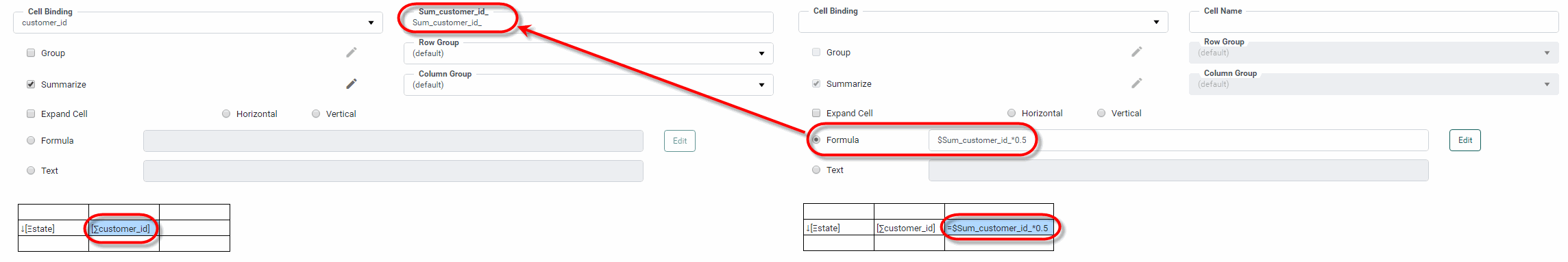
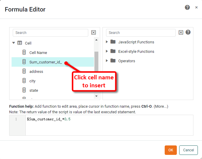
You can insert this reference easily by selecting the field name from the ‘Cell’ folder in the editor.

Freehand Table Cell Reference2 1

Extract a Query Column

To run a query in script, see Run a Query from Script. To retrieve an array of all values in a given field (column) from the query result set q, use the field name:

q['state'];

The following example illustrates this approach.

Example 1. Reference query column

Consider the sample ‘customers’ query. In this example, you will extract all the values under the ‘state’ column and use them to populate a Freehand table. Follow the steps below.

The ‘customers’ Data Worksheet can be found in Sample Queries. You may need to download the examples.zip file from GitHub into your environment. (This requires access to Enterprise Manager.) See Import and Export Assets for instructions on how to import.

Press the ‘Create’ button in the Visual Composer toolbar and select ‘New Dashboard’ button . This opens the ‘New Dashboard’ dialog box.
Press OK to close the dialog box and create the new Dashboard. (Do not select any data source.)
Press the ‘Options’ button in the Dashboard toolbar, and select the Script tab. Select the ‘onInit’ option at the bottom and enter the following script:
```
var q = runQuery('ws:global:Examples/customers')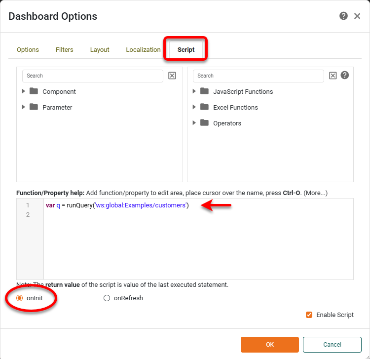
```
This executes the ‘customers’ query in the onInit script. (See Run a Query from Script for more details.)
Press OK to close the ‘Dashboard Options’ dialog box.
Drag the ‘Freehand Table’ component from the Toolbox panel into the Dashboard. This opens the Table Editor.
Click on cell[1,0] in the Table (second row, first column) to select it.
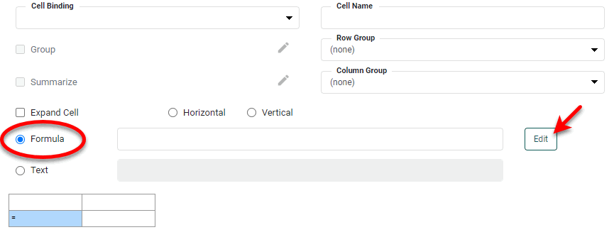
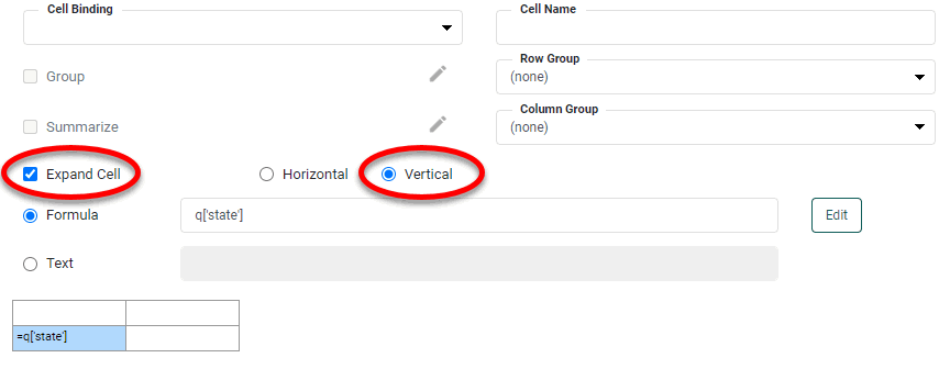
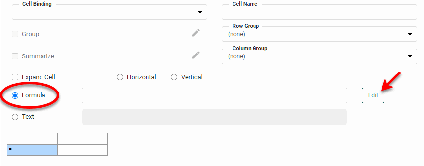
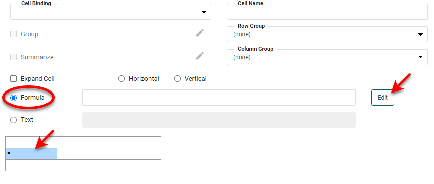
Select the ‘Formula’ option and press the Edit button.
Enter the following formula in the Formula Editor:
```
q['state']
```
This extracts the entire ‘state’ column from the ‘customers’ query to populate the table.
Press OK to close the Formula Editor.
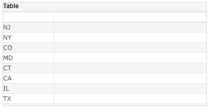
Select ‘Expand Cell’ and choose ‘Vertical’. (This causes the extracted data to fill down vertically.)

Observe that the table is populated with all the records from the ‘state’ column of the ‘customers’ query.

To return just the unique values in the ‘state’ column, change the script from q['state'] to toList(q['state']).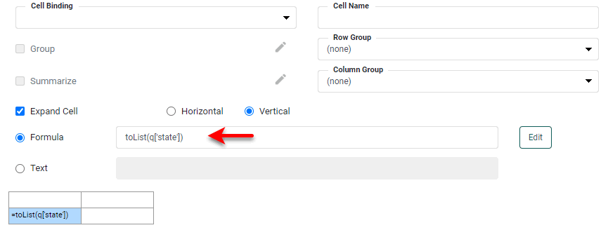

Derive Data from Query Columns

To run a query in script, see Run a Query from Script. In some cases you may want to perform operations on existing query columns to obtain the desired result. To do this, modify the formula by placing ‘=’ in front of the expression string. The following example illustrates this approach.

Example 2. Derive Data from Query Columns

Consider the sample ‘customers’ Data Worksheet. In this example, you will create a derived result that concatenates the value in the ‘state’ field with the value in the ‘zip’ field within a Freehand Table. Follow the steps below.

Press the ‘Create’ button in the Visual Composer toolbar and select ‘New Dashboard’ button . This opens the ‘New Dashboard’ dialog box.
Press OK to close the dialog box and create the new Dashboard. (Do not select a data source.)
Press the ‘Options’ button in the Dashboard toolbar, and select the Script tab. Select the ‘onInit’ option at the bottom and enter the following script:
```
var q = runQuery('ws:global:Examples/customers')
```
This executes the ‘customers’ data block in the onInit script. (See Run a Query from Script for more details.)
Press OK to close the ‘Dashboard Options’ panel.
Drag the ‘Freehand Table’ component from the Toolbox panel into the Dashboard. This opens the Table Editor.
Click on cell[1,0] in the table (second row, first column) to select it.
Select the ‘Formula’ option and press the Edit button.
Enter the following formula in the Formula Editor:
```
q['=state + ", " + zip'];
```
This concatenates the values in the ‘state’ column with the corresponding values in the ‘zip’ column.
Press OK to close the Formula Editor.
Select ‘Expand Cell’ and choose ‘Vertical’. (This causes the extracted data to fill down vertically.)

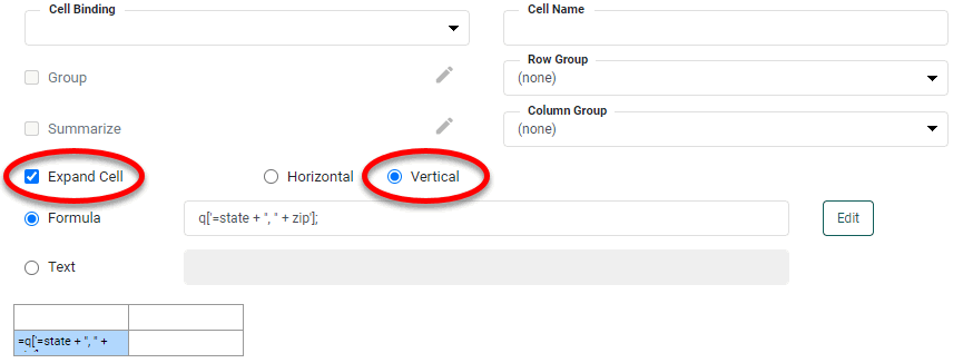
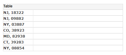
Observe that the table is populated with the concatenated values of ‘state’ and ‘zip’.

Extract Query Data with Field Filtering

You can filter values of a field (column) based on the values of other fields in the result set. To do this, use ‘@’ as the delimiter between the column name and the filtering expression and ‘:’ to introduce the values to filter. For example, to extract all values in a ‘company_name’ field where the corresponding value in the ‘state’ field is ‘NJ’, use the following formula:

q['company_name@state:NJ'];

This will yield a list of all the companies in New Jersey.

To retrieve a sub-table rather than an array, add an initial asterisk: q['*@state:NJ'];

To filter based on multiple fields, use ‘;’ as the delimiter between the filtering expressions. For example, to find all the companies within a certain city (New Brunswick) and state (NJ), adapt the formula as follows:

q['company_name@state:NJ;city:New Brunswick'];

If the filtering expression is based on a derived field (Derive Data from Query Columns), place ‘=’ in front of the expression. For example, to find all the companies within a certain ‘state, zip’ pair, adapt the formula as follows:

q['company_name@=state + ", " + zip:NJ, 08854'];

If the column name contains a space, use the rowValue operator:

q['company_name@=rowValue["US State"] + ", " + zip:NJ, 08854'];

The above examples use literal values (e.g., ‘NJ’, ‘New Brunswick’) in the condition. To use cell references in place of literal values, see Filter Query Based on Cell Value.

Extract Query Data with Expression Filtering

You can filter values in a column based on a conditional expression. Use ? as the delimiter between the filtering expression and the column name. For example, to extract all the values in the ‘company_name’ field where the corresponding value in the ‘customer_id’ field is between 20 and 30, use the following formula:

q['company_name?customer_id > 20 && customer_id < 30'];

Note, however, that while expression filtering can often be used to achieve the same result as field filtering, field filtering is better optimized. See Extract Query Data with Field Filtering for more details.

Extract Query Data with Index Filtering

You can filter values in a column based on a range of row indexes. For example, to extract the first five records from a ‘company_name’ column, use the following formula:

q['[0,company_name]:[4, company_name]'];

An asterisk ‘*’ in place of the row index represents the last row in the result set.

Filter Query Based on Cell Value

When extracting data from a query, you can use cell references as the filtering parameters. This is particularly useful when the table has multiple levels of row/column headers, and you want to filter the child level based on the parent level.

Example 3. Walkthrough

In this example, you will create a Freehand Table (based on the ‘customers’ query) with a two-level row header consisting of states and the cities within each state. Follow the steps below:

Press the ‘Create’ button in the Visual Composer toolbar and select ‘New Dashboard’ button . This opens the ‘New Dashboard’ dialog box.
Press OK to close the dialog box to create the new Dashboard. (Do not select any data source in the ‘New Dashboard’ dialog box.)
Press the ‘Options’ button in the toolbar, and select the Script tab. Select the ‘onInit’ option at the bottom and enter the following script:
```
var q = runQuery('ws:global:Examples/customers')
```
This executes the ‘customers’ data block in the onInit script. (See Run a Query from Script for more details.)
Press OK to close the ‘Dashboard Options’ panel.
Drag the ‘Freehand Table’ component from the Toolbox panel into the Dashboard. Press the ‘Edit’ button to open the Table Editor.
Right-click on the rightmost column and select ‘Append Column’ from the menu. The table should now have three columns.
Right-click on the bottom row and select ‘Insert Rows/Columns’ from the menu. Insert two rows at the bottom of the table.

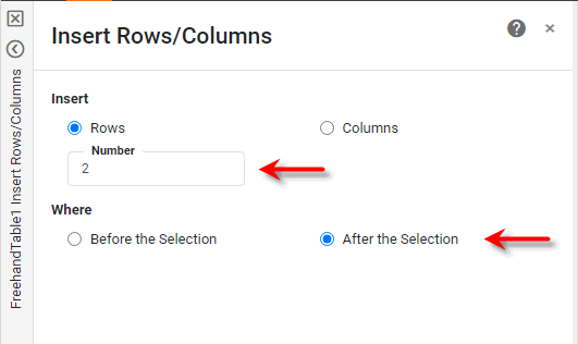
The table should now have four rows and three columns.
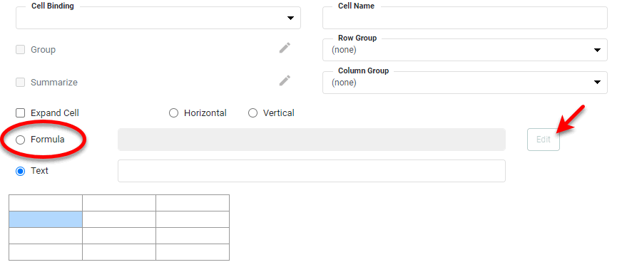
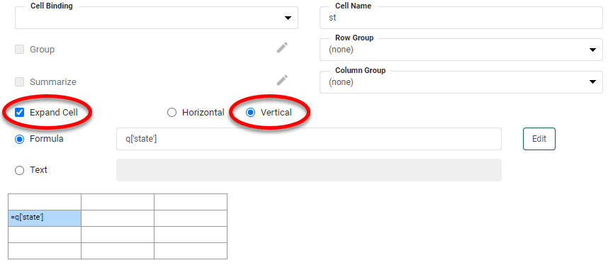
Click on cell[1,0] in the Table (second row, first column) to select it.
Select the ‘Formula’ option and press the Edit button.
Enter the following formula in the Formula Editor:
```
q['state']
```
This extracts the entire ‘state’ column from the ‘customers’ query to populate the table.
Press OK to close the Formula Editor.
Select ‘Expand Cell’ and choose ‘Vertical’. (This causes the extracted data to fill down vertically.)
In the ‘Cell Name’ field, enter ‘st’ as the cell name.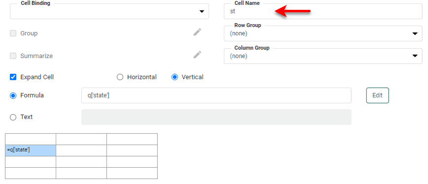
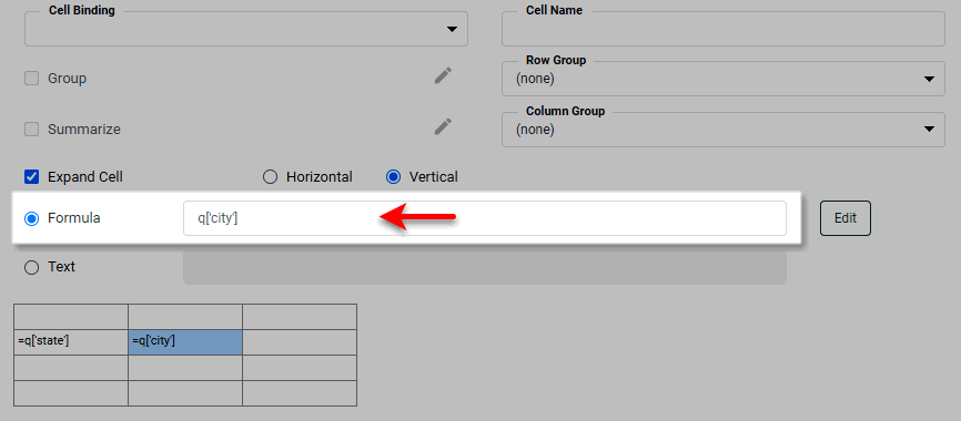
Select cell[1,1] in the table (second row, second column).
Select the ‘Formula’ option, and enter the following formula in the Formula Editor:
```
q['city']
```
This extracts the entire ‘city’ column from the ‘customers’ query.
Select ‘Expand Cell’ and choose ‘Vertical’.
In the ‘Cell name’ field, enter ‘ct’ as the cell name.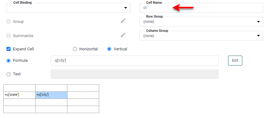
Press the ‘Finish’ button to close the Editor. Observe that the table is now populated with states and cities.

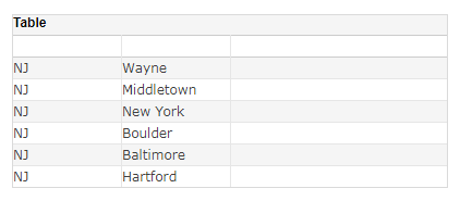
However, the second column lists all the cities next to each state, not only the cities that reside within the specific state. To filter the cities based on the state values, include a field-filtering condition with a reference to the cell ‘st’, as described below.
Press the ‘Edit’ button in the Table title bar to reopen the Table Editor.
Select cell[1,1] and change the formula from q['city'] to q['city@state:$st']. This returns only values from the ‘city’ field where the corresponding ‘state’ value is equal to the value in the table cell named ‘st’.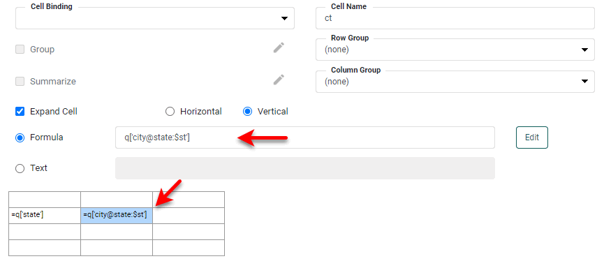

When making comparisons with 'null', use the syntax $st['.'] to reference the cell value.
Press the ‘Finish’ button to close the Editor. View the resulting table.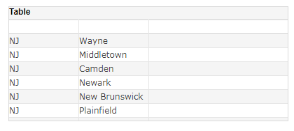

Notice that the table now lists only those cities that correspond to the given state. To further restrict the table’s data to display only unique values of city and state (i.e., to remove duplicates), modify the two formulas to use the toList() function:
```
// Cell[1,0]:
toList(q['state'])

// Cell[1,1]:
toList(q['city@state:$st'])
```

Use Cell Values in Summary Formulas

This section provides an example of using cell references in summary formulas.

Example 4. Walkthrough

Consider the formula table from the example in Filter Query Based on Cell Value. It consists of a two-level row header listing states and cities within each state. In the following example, you will add a formula to count the number of customers within each city.

Press the ‘Edit’ button in the Table title bar to reopen the Table Editor.
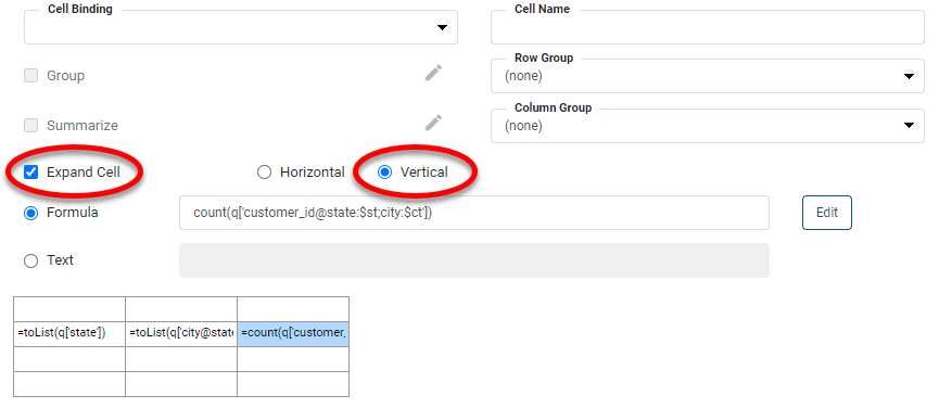
Select cell[1,2] (second row, third column), select the ‘Formula’ option, and add the following formula:
```
count(q['customer_id@state:$st;city:$ct'])
```
This formula counts all the customers within the given city and state.
Select the ‘Expand Cell’ option and choose the ‘Vertical’ option.
Press the ‘Finish’ button to close the Editor. The Table now displays a count of customer IDs within each city and state.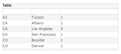

Group Numbering

To obtain the sequence number of an element within an expanding cell, use the ‘#’ qualifier. (This is useful when you wish to add numbering to row/column headers.)

Example 5. Group numbering

Consider the Freehand Table from the example in Use Cell Values in Summary Formulas. You will now add numbering for the expanding row header cell ‘st’.

Press the ‘Edit’ button in the Table title bar to reopen the Table Editor.
Right-click any cell in the first column and select Column Insert Column from the context menu. This adds a new column to the left.
Select cell[1,0] (second row) in the newly inserted column, select the ‘Formula’ option, and add the following formula:
```
$st['#'] + 1
```
Do not set any cell expansion. Note that group indexing starts with 0. The formula adds 1 to the index so that the first group has value 1.
Press the ‘Finish’ button to close the Editor. The table now displays the state group number in the first column. (You may need to resize the table to see all the columns.)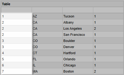

Note that the groups numbers are repeated for each instance of the state. To merge these repeated instances together, continue with the steps below.
Press the ‘Edit’ button in the Table title bar to reopen the Table Editor.
Select cell[1,0] (second row, first column).
Select the Option tab. Enable ‘Merge expanded cells’, and select ‘st’ from the ‘Row Group’ menu.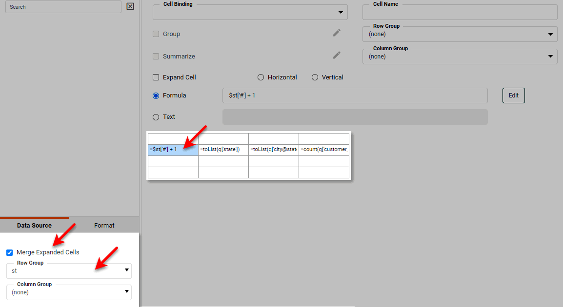
Select cell[1,1] (second row, second column).
In the bottom left panel, enable ‘Merge expanded cells’ and select ‘st’ from the ‘Row Group’ menu.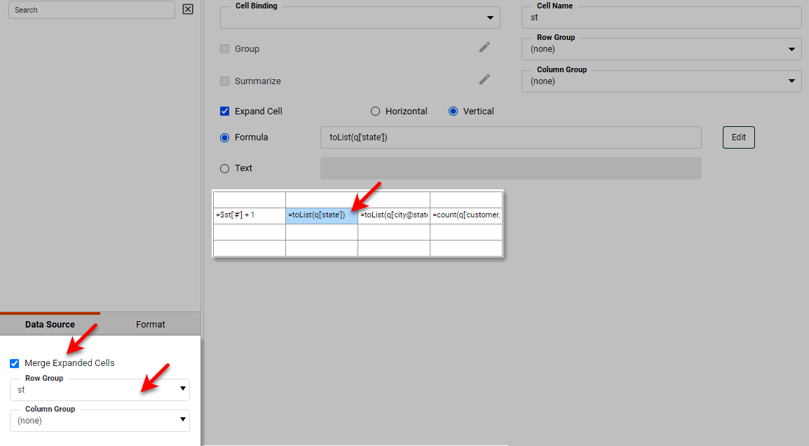
Press the ‘Finish’ button to close the Editor. Note how repeated states and group numbers have been merged together.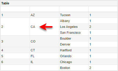
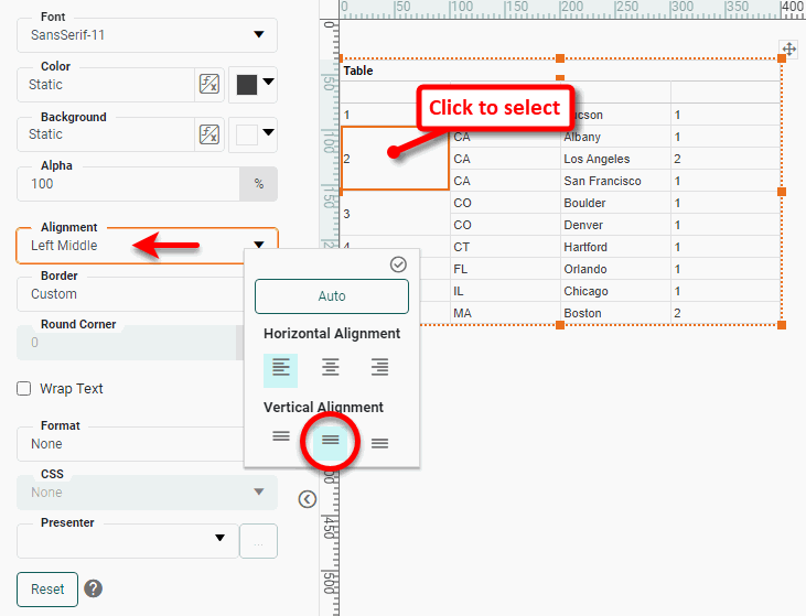
To vertically align these values within their cells, click on a cell to select it, and select the Format tab in the left panel if Visual Composer. Choose ‘Middle’ from the ‘Vertical Alignment’ property.

Reference a Cell with Relative Parent Group

Relative cell referencing is used primarily when comparing different summary cells with respect to their header cell. For example, you might want to find the difference between the total sales for the current year and the previous year. The syntax for relative cell referencing is as follows:

$cellName['grpName:+/-relative_index']

// Examples:
$sales['state:-1']
$sales['yr:+1']

Here, $cellName is the name of the cell/column containing the value(s) to be compared, and grpName is name of the cell/column that indexes the different values.

Example 6. Reference cell with relative parent group

In this example, you will find the difference in sales between successive fiscal years. Follow the steps below:

The 'Sales Explore' Data Worksheet can be found in Examples. You may need to download the examples.zip file from GitHub into your environment. (This requires access to Enterprise Manager.) See Import and Export Assets for instructions on how to import.

Press the ‘Create’ button in the Visual Composer toolbar and select ‘New Dashboard’ button . This opens the ‘New Dashboard’ dialog box.
Press OK to close the dialog box and create the new Dashboard. (Do not select any data source in the ‘New Dashboard’ dialog box.)
Press the ‘Options’ button in the toolbar, and select the Script tab. Select the ‘onInit’ option at the bottom and enter the following script:
```
var q = runQuery('ws:global:Examples/Sales Explore')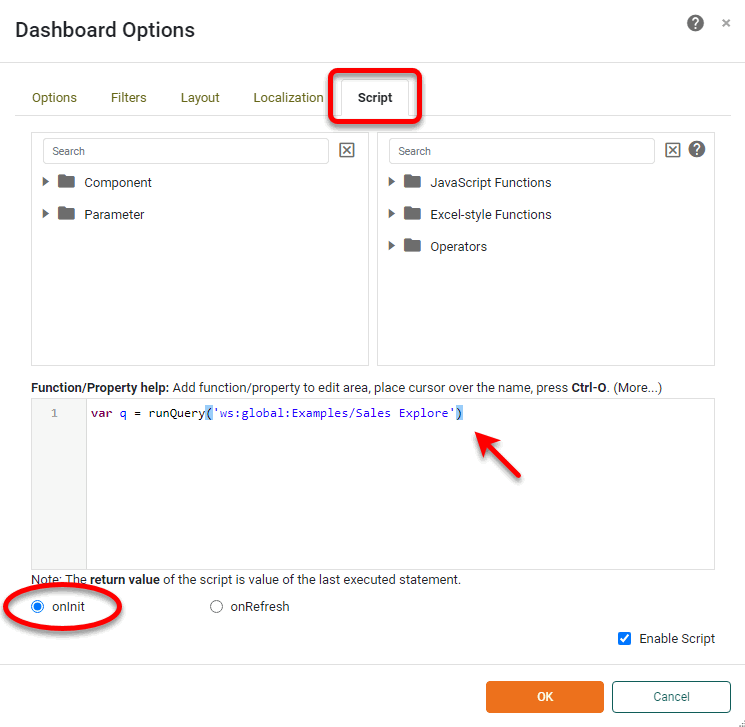
```
This executes the ‘Sales Explore’ Data Worksheet in the onInit script. (See Run a Query from Script for more details.)
Press OK to close the ‘Dashboard Options’ panel.
Drag the ‘Freehand Table’ component from the Toolbox panel into the Dashboard. Press the ‘Edit’ button to open the Table Editor.
Right-click on the rightmost column and select ‘Append Column’ from the menu. The table should now have three columns.
Right-click on the bottom row and select ‘Append Row’ from the menu. The table should now have three rows and three columns.
Click on cell[1,0] in the table (second row, first column) to select it.
Select the ‘Formula’ option and press the Edit button.
Enter the following formula in the Formula Editor:
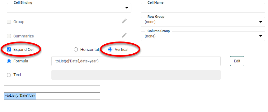
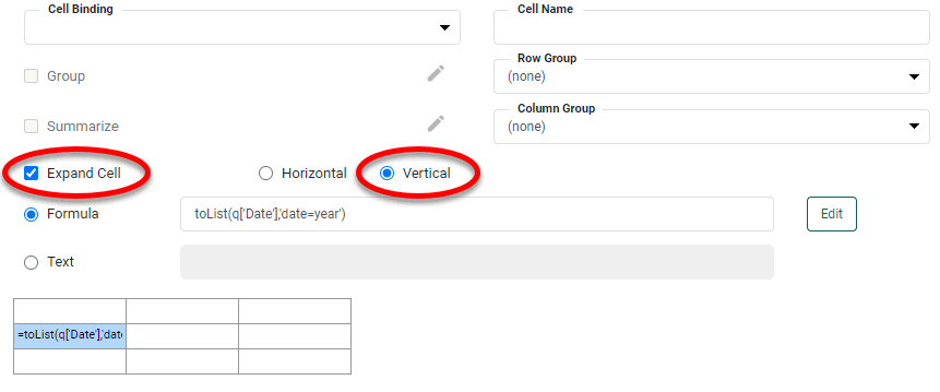
```
toList(q['Date'],'date=year')
```
This extracts the entire ‘Date’ column from the ‘Sales Explore’ Data Worksheet and groups the dates by year.
Press OK to close the Formula Editor.
Select ‘Expand Cell’ and choose ‘Vertical’. (This causes the extracted data to fill down vertically.)
In the ‘Cell Name’ field, enter ‘yr’ as the cell name.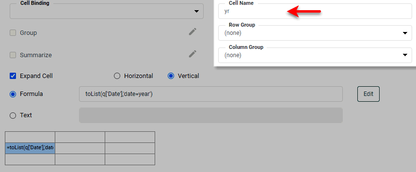
Select cell[1,1] in the table (second row, second column). Select the ‘Formula’ option, and enter the following formula:
```
sum(q['Total@=year(field["Date"]):$yr'])
```
This formula means “For each year in cell ‘yr’, find the values in the ‘Date’ field within that year, and sum the ‘Totals’ for those dates.” Effectively, this calculates the total revenue generated for a given year.
In the ‘Cell Name’ field, enter ‘tot’ as the cell name.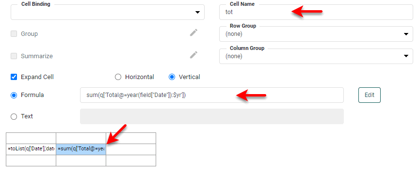
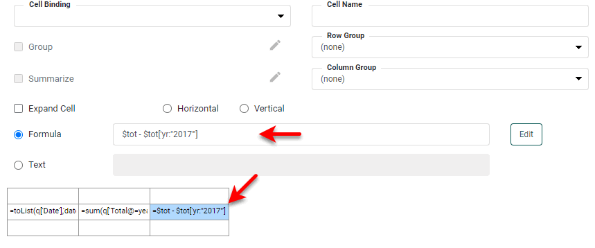
Select cell[1,2] (second row, third column). Select the ‘Formula’ option, and enter the following formula.
```
$tot - $tot['yr:-1']
```
This formula uses relative cell referencing to calculate the difference between the total revenue (computed in the column named ‘tot’) of the current year and the previous year. The table should appear as shown below.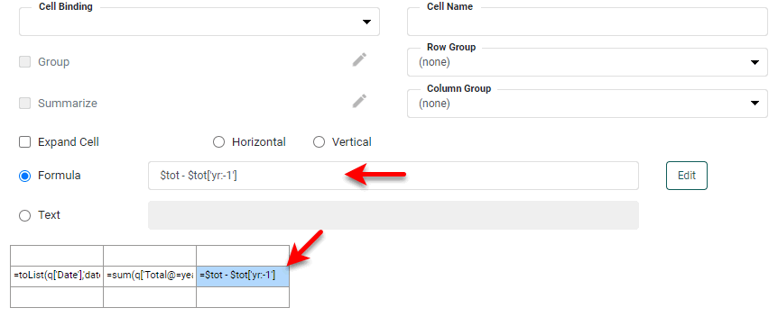
Press the ‘Finish’ button to close the Editor. The resulting table displays totals by year, as well as the difference between successive years’ totals.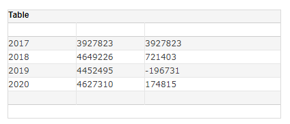

Reference a Cell with Absolute Parent Group

To refer to a summary cell in another header group, use the absolute value of the header group, as shown below:

$cellName['grpName:absolute_value']

// Examples:
$sales['state:NJ']
$sales['yr:"2011"'] // specify numeric values in quotes

Here, $cellName is the name of the cell/column containing the value(s) to be compared, and grpName is name of the cell/column that indexes the different values.

Example 7. Reference cell with absolute parent group

In this example, you will find the relative sales for each year compared to the fixed year 2017. Follow the steps below:

Press the ‘Create’ button in the Visual Composer toolbar and select ‘New Dashboard’ button . This opens the ‘New Dashboard’ dialog box.
Press OK to close the dialog box and create the new Dashboard. (Do not select any data source in the ‘New Dashboard’ dialog box.)
Press the ‘Options’ button in the toolbar, and select the Script tab. Select the ‘onInit’ option at the bottom and enter the following script:
```
var q = runQuery('ws:global:Examples/Sales Explore')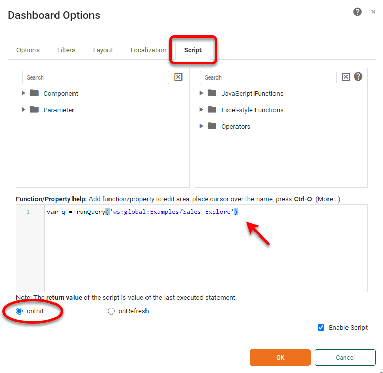
```
This executes the ‘Sales Explore’ query in the onInit script. (See Run a Query from Script for more details.)
Press OK to close the ‘Dashboard Options’ panel.
Drag the ‘Freehand Table’ component from the Toolbox panel into the Dashboard. Press the to open the Table Editor.
Right-click on the rightmost column and select ‘Append Column’ from the menu. The table should now have three columns.
Right-click on the bottom row and select ‘Append Row’ from the menu. The table should now have three rows and three columns.
Click on cell[1,0] in the table (second row, first column) to select it.
Select the ‘Formula’ option and press the Edit button.
Enter the following formula in the Formula Editor:
```
toList(q['Date'],'date=year')
```
This extracts the entire ‘Date’ column from the ‘Sales Explore’ Data Worksheet and groups the dates by year.
Press OK to close the Formula Editor.
Select ‘Expand Cell’ and choose ‘Vertical’. (This causes the extracted data to fill down vertically.)
In the ‘Cell Name’ field, enter ‘yr’ as the cell name.
Select cell[1,1] in the table (second row, second column). Select the ‘Formula’ option, and enter the following formula:
```
sum(q['Total@=year(field["Date"]):$yr'])
```
This formula means “For each year in cell ‘yr’, find the values in the ‘Date’ field within that year, and sum the ‘Totals’ for those order dates.” Effectively, this calculates the total revenue generated for a given year.
In the ‘Cell Name’ field, enter ‘tot’ as the cell name.
Select cell[1,2] (second row, third column). Select the ‘Formula’ option, and enter the following formula.
```
$tot - $tot['yr:"2017"']
```
This formula uses absolute cell referencing to calculate the difference between the total revenue (computed in the column named ‘tot’) of the current year and the year 2017. The table should appear as shown below:
Press the ‘Finish’ button to close the Editor. The resulting table displays totals by year, as well as the difference between each year’s total and the total for 2017.

Reference a Cell with Absolute Parent Group

To refer to a summary cell in another header group, use the absolute value of the header group, as shown below:

$cellName['grpName:absolute_value']

//Examples:
$sales['state:NJ']
$sales['yr:"2011"'] // specify numeric values in quotes

Here, $cellName is the name of the cell/column containing the value(s) to be compared, and grpName is name of the cell/column that indexes the different values.

Example 8. Reference cell with absolute parent group

In this example, you will find the relative sales for each year compared to the fixed year 2017. Follow the steps below:

Press the ‘Create’ button in the Visual Composer toolbar and select ‘New Dashboard’ button . This opens the ‘New Dashboard’ dialog box.
Press ‘OK’ to close the dialog box and create the new Dashboard. (Do not select any data source in the ‘New Dashboard’ dialog box.)
Press the in the toolbar, and select the Script tab. Select the ‘onInit’ option at the bottom and enter the following script:
```
var q = runQuery('ws:global:Examples/Sales Explore')
```
This executes the ‘Sales Explore’ query in the onInit script. (See Run a Query from Script for more details.)
Press OK to close the ‘Dashboard Options’ panel.
Drag the ‘Freehand Table’ component from the Toolbox panel into the Dashboard. Press the to open the Table Editor.
Right-click on the rightmost column and select ‘Append Column’ from the menu. The table should now have three columns.
Right-click on the bottom row and select ‘Append Row’ from the menu. The table should now have three rows and three columns.
Click on cell[1,0] in the table (second row, first column) to select it.
Select the ‘Formula’ option and press the Edit button.
Enter the following formula in the Formula Editor:
```
toList(q['Date'],'date=year')
```
This extracts the entire ‘Date’ column from the ‘Sales Explore’ Data Worksheet and groups the dates by year.
Press OK to close the Formula Editor.
Select ‘Expand Cell’ and choose ‘Vertical’. (This causes the extracted data to fill down vertically.)
In the ‘Cell Name’ field, enter ‘yr’ as the cell name.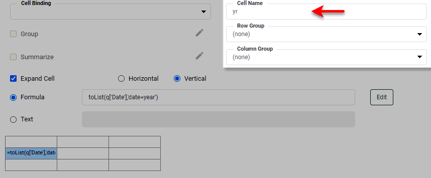
Select cell[1,1] in the table (second row, second column). Select the ‘Formula’ option, and enter the following formula:
```
sum(q['Total@=year(field["Date"]):$yr'])
```
This formula means “For each year in cell ‘yr’, find the values in the ‘Date’ field within that year, and sum the ‘Totals’ for those order dates.” Effectively, this calculates the total revenue generated for a given year.
In the ‘Cell Name’ field, enter ‘tot’ as the cell name.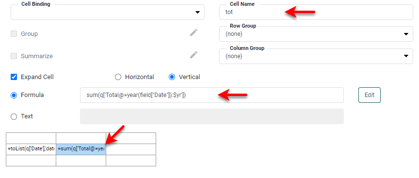
Select cell[1,2] (second row, third column). Select the ‘Formula’ option, and enter the following formula.
```
$tot - $tot['yr:"2017"']
```
This formula uses absolute cell referencing to calculate the difference between the total revenue (computed in the column named ‘tot’) of the current year and the year 2017. The table should appear as shown below:
Press the ‘Finish’ button to close the Editor. The resulting table displays totals by year, as well as the difference between each year’s total and the total for 2017.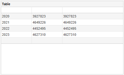

Reference a Cell with Parent Group as an Expression

To specify a referenced group using a JavaScript expression, prefix the expression string with ‘=’, as shown below:

$company['state:=iif($type == "T", $state, $province)']

The syntax of the iif function used above is CALC.iif(condition, value_if_true, value_if_false).